
Introduction LabVIEW (Laboratory Virtual Instrument Engineering Workbench) is a graphical programming language that integrates all the functions of the hardware and data acquisition card that meet the GPIB, VXI, RS-232, and RS-485 protocols. It also has built-in ease of application of TCP/IP, ActiveX. Other software standard library functions. Using LabVIEW can easily create a variety of virtual instruments.
The spectrum analyzer is an essential means for measuring radio signals. It is a common tool for the research and development, production, and inspection of electronic products. It is widely used and is called an engineer's RF multimeter. The front-end circuit of the traditional spectrum analyzer is a tunable receiver in a certain bandwidth, and the input signal is output by the low-pass filter after frequency conversion by the frequency converter. The filtered output signal is used as the vertical component and the frequency is used as the horizontal component. The coordinate graph is plotted on the oscilloscope screen, which is the spectrum of the input signal. Because the frequency converter can reach a wide frequency, such as 30Hz-30GHz, and can be extended to more than 100GHz with an external mixer, the frequency-difference analyzer is one of the most widely used frequency measurement instruments, regardless of continuous signal or modulation measurement. Signals, spectrum analyzers are ideal measurement tools. However, the traditional spectrum analyzer can only measure the amplitude of the frequency, lack of phase information, it is a scalar instrument, and it is bulky. Using LabVIEW's powerful virtual instrument development capabilities, modern spectrum analyzers based on fast Fourier transform (FFT) can be implemented. Digital signals are directly sampled by an analog/digital converter (ADC) and processed by FFT. Obtaining the spectrum map can solve the disadvantages of the traditional spectrum analyzer, such as expensive and inconvenient to carry.
1. The overall design of the virtual spectrum analyzer The virtual spectrum analyzer consists of a data acquisition card, a computer, and application software developed on LabVIEW that runs on it, as shown in Figure 1.

The virtual spectrum analyzer uses the analog input and analog output of the data acquisition card to generate the desired excitation signal using the analog output function and add it to the network under test. Then, the two analog input channels are used to combine the excitation signal with The response signal of the network output end is collected into the computer at the same time. After being processed, it forms the amplitude-frequency and phase-frequency characteristics, and is displayed on the computer screen. Finally, the signal generated by the simulation is analyzed, and the amplitude of the analog signal is output on the computer screen. / Phase frequency characteristics.
2. Composition and function of virtual spectrum analyzer 2.1 Virtual instrument and spectrum analyzer The virtual spectrum analyzer designed in this paper consists of three sub-modules: periodic signal generator, filter, and amplitude/frequency/frequency characteristics and spectrum analysis results. . The signal generator submodule generates two analog input signals, one is a sine signal with adjustable frequency, phase, and amplitude, and the other is a cosine signal with adjustable frequency, phase, and amplitude. Finally, a signal synthesizer is used to mix the two signals. As a generated 2-way analog signal, the spectrum analysis and filter sub-module utilizes LabVIEW's powerful digital signal processing function to filter, window, and FFT the processing data of this group to obtain the real part spectrum and the imaginary part spectrum of the signal. The most important is to obtain the amplitude-frequency characteristic curve and the phase-frequency characteristic curve of the signal; in the result module of spectrum analysis, the spectrum of the generated signal is analyzed, and the parameters such as the RMS value and the signal average value in one period are Save to text file when the system exits. Among them, in the filter setting, the filtering passing mode and the cutoff frequency can be controlled, and finally the spectrum analysis result is displayed. When the system exits, it prompts to save the current data to a text file.
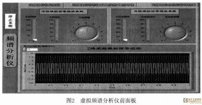
The front panel of the virtual spectrum analyzer is divided into three parts: periodic signal generators, periodic signal filters, and amplitude/phase frequency characteristics and periodic signal spectrum analysis results, as shown in Figure 2. The figure shows the interface of the periodic signal generator. In the figure, the sine wave and cosine wave signals can be changed by the mouse drag and rotate buttons to change the frequency, amplitude and phase of the signal. When dragging, it can be seen that the "2 channels of original analog signal waveform" below will change, and the maximum value of the abscissa axis will also change. This function can be realized by calling the "XScaleControl.VI" described later in the program; for the "periodic signal filter and amplitude/phase frequency characteristics" and "periodic signal spectrum analysis results", the two functional module interfaces are limited in length. No longer.
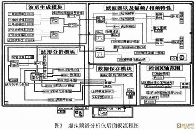
The back panel of the virtual spectrum analyzer consists of five sub-modules: the waveform generation module, the waveform analysis module, the control of the X-axis range, the filter, and the amplitude/frequency/phase-frequency characteristics and data storage module, as shown in Figure 3.
2.2 The design of the virtual spectrum analyzer sub-module (1) Waveform generation sub-module To perform spectrum analysis, we must first generate an analog signal. This article takes two sub-modules of the system: Trianglewaveform.VI and Sinewaveform.VI to generate two analog input signals. In order to achieve the adjustment of the frequency, phase and amplitude of the analog signal, several control inputs have been added, as shown in Figure 4 and Figure 5.
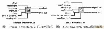
In Figure 4 and Figure 5, the input pin and output pin are exactly the same, "offset" refers to the offset of the waveform, generally not set; "resetsignal" is a Boolean input control, if loaded as True You can reset the waveform. If it is False, the waveform is not reset. "frequency" refers to the frequency of the generated signal; "amplitude" refers to the amplitude of the signal you want to generate; "phase" refers to the phase of the generated signal; "errorin" and "errorout" refers to the input and output when the program has an exception; "samplinginfo" refers to the sampling rate of the signal to be generated. The default setting is 1000, that is, 1000 points per second; "DutyCycle" is the duty cycle. , refers to the ratio of the duration of a positive pulse to the total period of a pulse in a string of ideal pulse trains (such as a square wave).
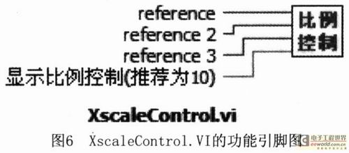
(2) Controlling the X-axis range The sub-module XscaleControl.VI is used to implement the dynamic control waveform X-axis range. There are 4 input pins, 3 of which are reference reference inputs and one is a constant input pin. With an increase in the frequency of the input signal, if the X-axis range of the output waveform is fixed to be 1, then the waveform display is too dense, resulting in no clear picture at all. Therefore, when the frequency increases, the x-axis range of the waveform is relatively reduced. To make the waveform display more clearly. Three reference input pins refer to the sine wave frequency, triangle wave frequency, and waveform control WaveformGraph property controls. The internal working principle is that when the sine wave frequency and the triangular waveform frequency are greater than 10 Hz, the reciprocal of the larger of the two frequencies is used as the maximum value of the abscissa axis of the waveform control WaveformGraph. It realizes the function that the waveform is still clear when the frequency of the analog signal increases, thus realizing the dynamic control of the range of the x-axis of the waveform control.
(3) Waveform Analysis Sub-module LabVIEW provides a wealth of waveform spectrum analysis tools, the most typical is Amplitude and LevelMeasurement.VI, its storage path is in the rear panel Functions -> SignalAnalysis, parameter dialog box is divided into four areas, respectively AmplitudeMeasurements are required to be evaluated, results of current signal amplitude evaluation, input signal preview window (InputSignal), and windowed signal preview window (ResultSignal). Among them, the most important is Amplitude and LevelMeasurement.VI will automatically add this output port to its icon to determine which feature value to use for setting the item's settings. The spectrum analysis Amplitude and LevelMeasurement.VI function pins are shown in Figure 7.

This module has 3 input pins and 8 output pins. The three input pins are as follows: The "RestartAveraging" pin identifies whether to restart the selected averaging process. The default is False; the "Signals" pin is the input signal to be analyzed; the "errorin(noerror)" pin is A description of the error condition precedes execution into this VI; the eight output pins are described as follows: "RMS" pin refers to signal rms value; "PositivePeak" pin refers to positive peak; "errorout" pin refers to subVI. Output information at error execution; "CycleAverage" pin means average over one cycle; "CycleRMS" pin means rms value of one cycle; "Mean(DC)" pin means signal mean; "NegativePeak" pin Refers to the negative peak; the "PeaktoPeak" pin refers to the peak-to-peak value, which is the maximum amplitude value of the positive and negative directions of the input signal waveform.
By using the signals generated by the simulation as the input signal "Signals" of this VI, the generated signal can be analyzed to output some parameter information of the signal, such as the mean value of the signal, the peak value and the RMS value of one cycle, etc. .
Another typical signal analysis VI is FFTSpectrum (Real-Im). VI, the VI can calculate the fast Fourier transform spectrum of the input time domain signal, and return the real part spectrum and the imaginary part spectrum of the waveform respectively. It is also meaningful to analyze the real part spectrum and the imaginary part spectrum in practical applications. Fourier spectrum transform FFTSpectrum. The VI function pin is shown in Figure 8.
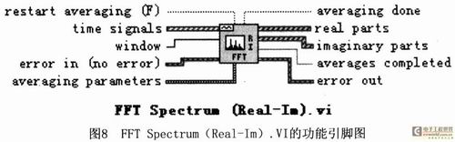
This module has 10 pins in total. The "restartaveraging(F)" pin is the same as the above-mentioned function, used to identify whether to restart the selected average processing; the "timesignals" pin identifies the input time domain signal; the "window" pin refers to the window setting. The windowing method includes a variety of different methods, such as Uniform, Hanning, Hamming, and Blackman; the "errorin(noerror)" pin and the "errorout" pin identify the input and output information when the error occurs in the execution of this VI. The "averaging parameters" pin refers to the average parameter of the input waveform signal; the "realparts" pin identifies the real part spectrum of the waveform, and the output can be described graphically by a graph image or a description of a bunch of parameters; "imaginaryparts" cited The imaginary spectrum of the input waveform of the toe is described in the same way as the real spectrum; the remaining two pins, the "averagingdone" pin and the "averagescompleted" pin, are generally not used, and are descriptions of some infrequent parameters of the input waveform.
(4) Filter and amplitude-frequency/phase-frequency characteristics sub-module The filter sub-module is in the Functions->SignalAnalysis sub-template. Its settings are divided into four areas, which are Filtering Type and two preview windows. And preview mode setting area (VIewMode). There are four types of filters, high pass, low pass, band pass, and smoothing filters. The first three are easy to understand, and the smoothing filter is mainly used to locally average the signal and eliminate periodic or white noise. Low-pass filter sub-module Filter. The functional pins of the VI are shown in Figure 9.

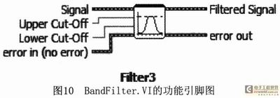
Bandpass filter sub-module BandFilter. The functional pins of the VI are shown in Figure 10. As the name implies, the bandpass filter means that the frequency can pass through a certain range of waveforms. It has one more pin, UpperCut-Off, than the low-pass filter in Figure 9.
(5) Data saving sub-module data saving sub-module ie SaveData. The VI function pin is shown in Figure 11. It processes the data you want to save into a unified format and saves it to a text file when the system exits.
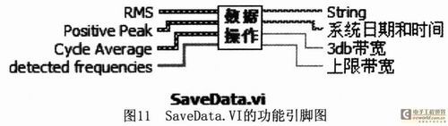
Of these, only two pins are the output, "string" and "system date and time", which represent the formatted output string and the current date and time of the system. A record format of the output "string" in the system automatic storage file is as follows:
"Cycle average: -0.258667 positive peak: 2.845332 signal rms value: 2.8453323 dB bandwidth: 392.968235.
August 21, 2007 12:21:32", where "period average" denotes the signal average of the waveform signal over one cycle; "positive peak" denotes the maximum amplitude value reached by the waveform signal; "signal rms The value "" indicates the value of the waveform signal calculated by the rms formula; "3dB bandwidth" indicates the width of the bandwidth obtained by the subVI; the last one represents the date and time of the record, which is mainly used by LabVIEW. The Format function, which is formatted into the same string "string" by a plurality of Chinese strings and a number through the Fromat function, in order to save the data when the system exits, because if you put the saved data into the while loop , it will cause the program to endless loop because it has been prompted to save the data.
In Figure 11, there are six input pins, where the "RMS" pin represents the periodic average of the signal, the "PositivePeak" pin represents the maximum positive peak, and the "CycleAverage" pin represents the signal rms," ​​detectedfrequencies "Pin is the detected frequency, and the "3db bandwidth" pin and the "Upper Bandwidth" pin are calculated by nesting a subVI, Compute3dbbandwidth.VI.
3. Conclusion Based on the LabVIEW programming environment, the virtual spectrum analyzer mainly implements two functions: time domain analysis and frequency domain analysis. The time domain analysis of the signal is mainly to measure the feature values ​​of the test signal after filtering. These feature values ​​represent some time domain features of the signal in a numerical value, which is the most simple and intuitive time domain description of the test signal. After the test signal is collected into the computer, the signal eigenvalue processing is performed in the test VI, and the characteristic value of the signal is visually represented on the front panel of the test VI, which can provide a user with test VI with a quick way to understand the change of the test signal. . The eigenvalues ​​of the signal are divided into amplitude eigenvalues, time eigenvalues ​​and phase eigenvalues. This paper designs the analysis of the amplitude eigenvalues.
The frequency domain analysis of the signal is based on the frequency domain description of the signal to estimate and analyze the signal composition and feature quantities. It is to study the frequency structure of the signal, that is, to obtain the distribution law of the amplitude and phase of its components according to the frequency, and establish various spectra with the frequency as the horizontal axis. For a periodic signal, it can be expanded into a Fourier coefficient, and its frequency spectrum is discrete, harmonic, and convergent; for a non-periodic signal, the frequency composition can be analyzed by its spectral density function, and its frequency spectrum has continuity.
Cylinder is the place where the fuel-air mixture is compressed and burned to convert chemical energy to heat and mechanical energy to make the bike go. Just like in any other internal combustion engine. The engine might have only one cylinder or many. More than four is rare, though.The cylinder is fired by a spark plug which creates a spark electrically from the battery .
It is the cylinder in an engine where the combustion takes place-..in vehicle the cylinder is just above the transmission. think of it as a syringe. the piston moves up and compresses the air fuel mixture and as a result combustion takes place. the piston is then pushed down. this up and down motion of the piston rotates the crankshaft which is connected to the transmission which transmits power to the wheels. there are various configurations of cylinders in an engine. in vehicle have single cylinder, parallel twin, v twin, L twin, inline 4, inline 3, inline 6, v4, flat twin. similarly in cars you get inline 3, inline4, inline6 , v6, v8, v10, w12. the number represents the no. of cylinders and the letter or prefix represents the configuration.
Motorcycle Cylinder,Cylinder Kit,Motorbike Engine Part,Motorcycle Engine Cylinder
LIXIN INDUSTRIAL & TRADE CO.,Limited , https://www.jmsparkplugs.com